Coursera's machine learning course (implemented in Python)
07 Jul 2015
Last week I started Stanford’s machine learning course (on Coursera). The course consists of video lectures, and programming exercises to complete in Octave or MatLab. Contrary to what Ng says, the most popular languages for data science seem to be Python, R or Julia (high level languages), and Java, C++ or Scala/Clojure (low level languages). Ryan Orban of Zipfian Academy recommends you learn one of both. I’ve never heard of people using MatLab outside of an academic context, so I’ve decided to attempt the exercises in Python.
Week two programming assignment: linear regression
The first assignment starts in week two and involves implementing the gradient descent algorithm on a dataset of house prices. At a theoretical level, gradient descent is an algorithm that is used to find the minimum of a function. That is, given a function that is defined by a set of parameters, gradient descent iteratively changes the parameter values, so that the function is progressively minimised. This ‘tuning’ algorithm is used for lots of different machine learning applications. In this exercise, we were shown how to use gradient descent to find the best fit for a linear regression.
I realise what I just said will sound like gobbledigook if you haven’t used gradient descent before! I hope this post will explain things better.
The scenario: food trucks
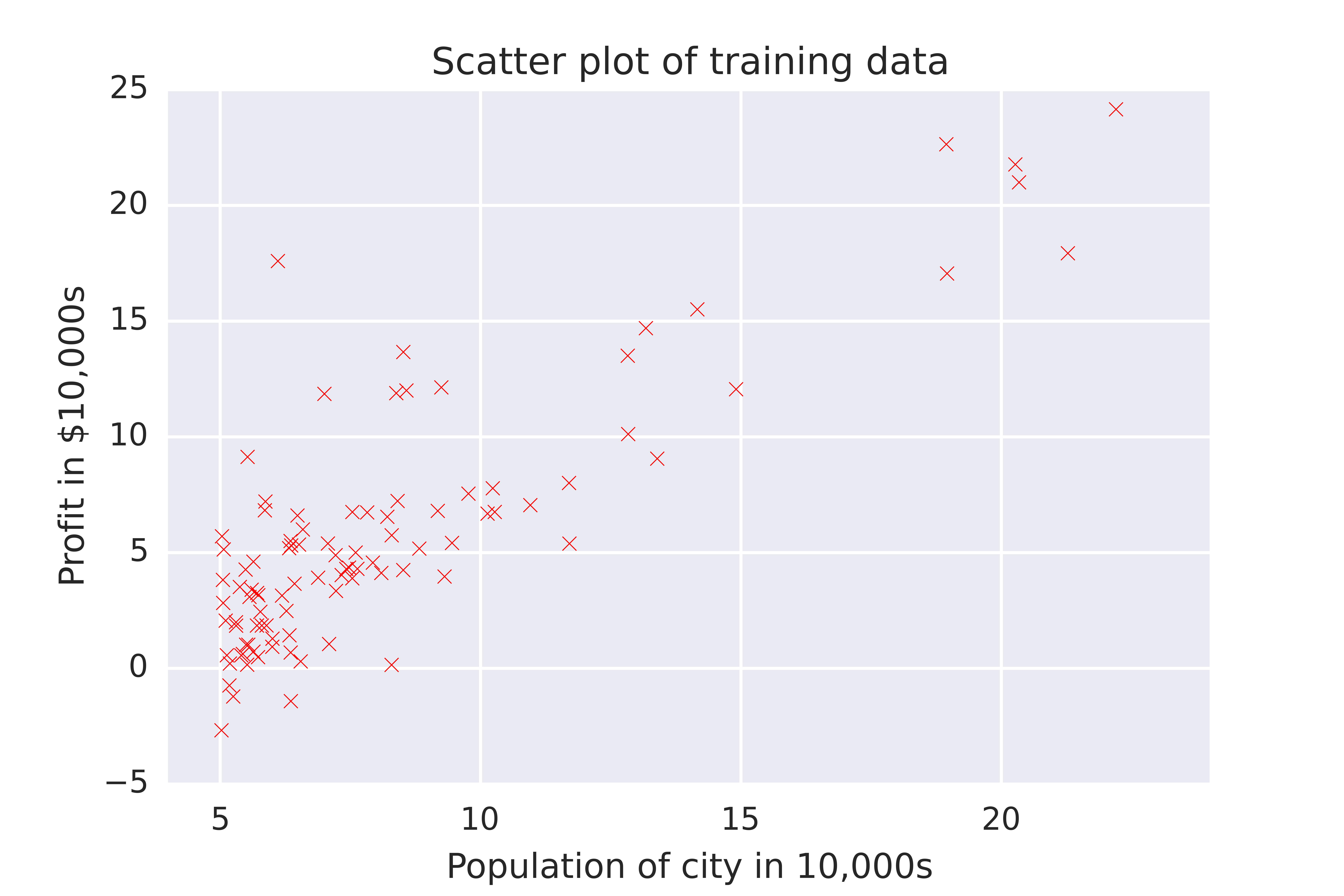
We were told to imagine that we are a CEO of a large food truck franchise and we are considering cities to send more food trucks (if I had a food truck franchise, my food trucks would serve pierogei). Obviously, we want to find a way to maximise our profit. Fortunately we already have food trucks dishing out hot dumplings in several cities, so we can examine the data from these and predict the profits of future trucks. Since we have this training dataset, this is a supervised learning rather than an unsupervised learning task. Our dataset includes the population sizes of the cities where we already have food trucks, and our profits from each of these cities. Since we only have one input variable (population size) per output variable that we’re trying to predict (profits), this is univariate (as opposed to multivariate) linear regression. Here’s what the data looks like on a scatter plot

As you can see, profits increase with increasing city size. But how can we predict how much profit future food trucks will make? We’ll have to fit a regression line summarises our past data.
The hypothesis function
The standard equation for a line (with just one variable, x) is:
We’ll use machine learning to help us to find values for m and c (that is, the values for the gradient and y-intercept of the line) that best describe the data. From now on, I’ll refer to c as \(\theta_0\) and m as \(\theta_1\) (this notation makes things easier when we start dealing with more than one variable). Our machine learning algorithm will come up with values for \(\theta_0\) and \(\theta_1\) that we’ll be able to use to plug into the linear equation, above, and so predict values of y (i.e. profit) for any values of x (i.e. population size) we so desire. In machine learning lingo, these outputs are called hypotheses. For linear regression with one variable, our hypothesis function will be of the form:
which you can see is just a different representation of the equation above.
The cost function
How can we assess how good a particular hypothesis is? For this we need something called a cost function (otherwise known as a loss function), which quantifies how much our prediction \(h_\theta(x)\) deviates from the actual value of \(y\). So we want to find the values for \(\theta_0\) and \(\theta_1\) that will make the output from our cost function as small as possible.
The cost function that we used here was the mean squared error:
Let’s break this down. We can see that the cost function, \(J\), takes the values of \(\theta_0\) and \(\theta_1\) as inputs. The term \(h_\theta(x^{(i)})-y^{(i)})\) is finding the difference between the hypothesis value (estimated profit, under the proposed values of \(\theta_0\) and \(\theta_1\) and the actual value of y (actual profit) for each of the examples in our training dataset (identified by the superscript \(i\)). This is our error value; the bigger the difference between the estimated and actual values, the larger the error.
We then square each of the error values (this makes them all positive) and add them together. Then we find the average of these values by dividing by \(\frac 1m\). We also multiply by \(\frac 12\), as this makes computation of the gradient descent (coming up next!) more convenient.
So, altogether the cost function computes half of the average of the sum of squared errors. Phew!
In Python, here’s how I programmed the cost function:
1
2
3
4
5
6
7
8
9
10
 # define a function that computes the cost function J()
 def costJ(X,y,theta):
    '''where X is a pandas dataframe of input features, plus a column of ones to accommodate theta 0;
    y is a vector that we are trying to predict using these features, and theta is an array of the parameters'''

    m = len(y)
    hypothesis = X.dot(theta)
    a = (hypothesis[0]-y)**2
    J = (1/(2*m)*sum(a))
    return J
Gradient descent
How can we efficiently find values of \(\theta_0\) and \(\theta_1\) that minimise the cost function, you cry? Here’s where gradient descent comes in. The gradient descent algorithm updates the values for \(\theta_0\) and \(\theta_1\) in the direction that minimises \(J(\theta_0, \theta_1)\):
The direction we should move to minimise the cost function is found by taking the derivative (the line tangent to) the cost function; this is what the term \(\frac{\partial}{\partial\theta_j} J(\theta_0,\theta_1)\) is doing. We then multiply this by the coefficient \(\alpha\) to work out how far we should move along this tangent. Update for both values of \(\theta_0\) and \(\theta_1\) before re-computing the cost function. Rinse and repeat until the output of the cost function reaches a steady plateau. The step sizes we take at each iteration towards the minimum is determined by \(\alpha\).
When applied specifically to linear regression, the gradient descent algorithm can be derived like this:
where \(\theta_0\) and \(\theta_1\) are updated simultaneously until convergence. (If it seems like I just skipped over that derivation, it’s because it’s really long and I don’t quite understand it yet.)
Here’s how my gradient descent algorithm looks in Python:
1
2
3
4
5
6
7
8
9
10
11
12
13
14
15
16
17
18
19
def gradDesc(X,y,theta,alpha,num_iters):
    '''Implement the gradient descent algorithm, where alpha is the learning rate and num_iters is the number of iterations to run'''

    #initiate an empty list to store values of cost function after each cycle
    Jhistory = []
    theta_update = theta.copy()

    for num_iter in range(num_iters):
        #these update only once for each iteration
        hypothesis = X.dot(theta_update)
        loss = hypothesis[0]-y

        for i in range(len(X.columns)):
            #these will update once for every parameter
            theta_update[i] = theta_update[i] - (alpha*(1.0/m))*((loss*(X.iloc[:,i])).sum())

        Jhistory.append(costJ(X,y,theta_update))

    return Jhistory, theta_update
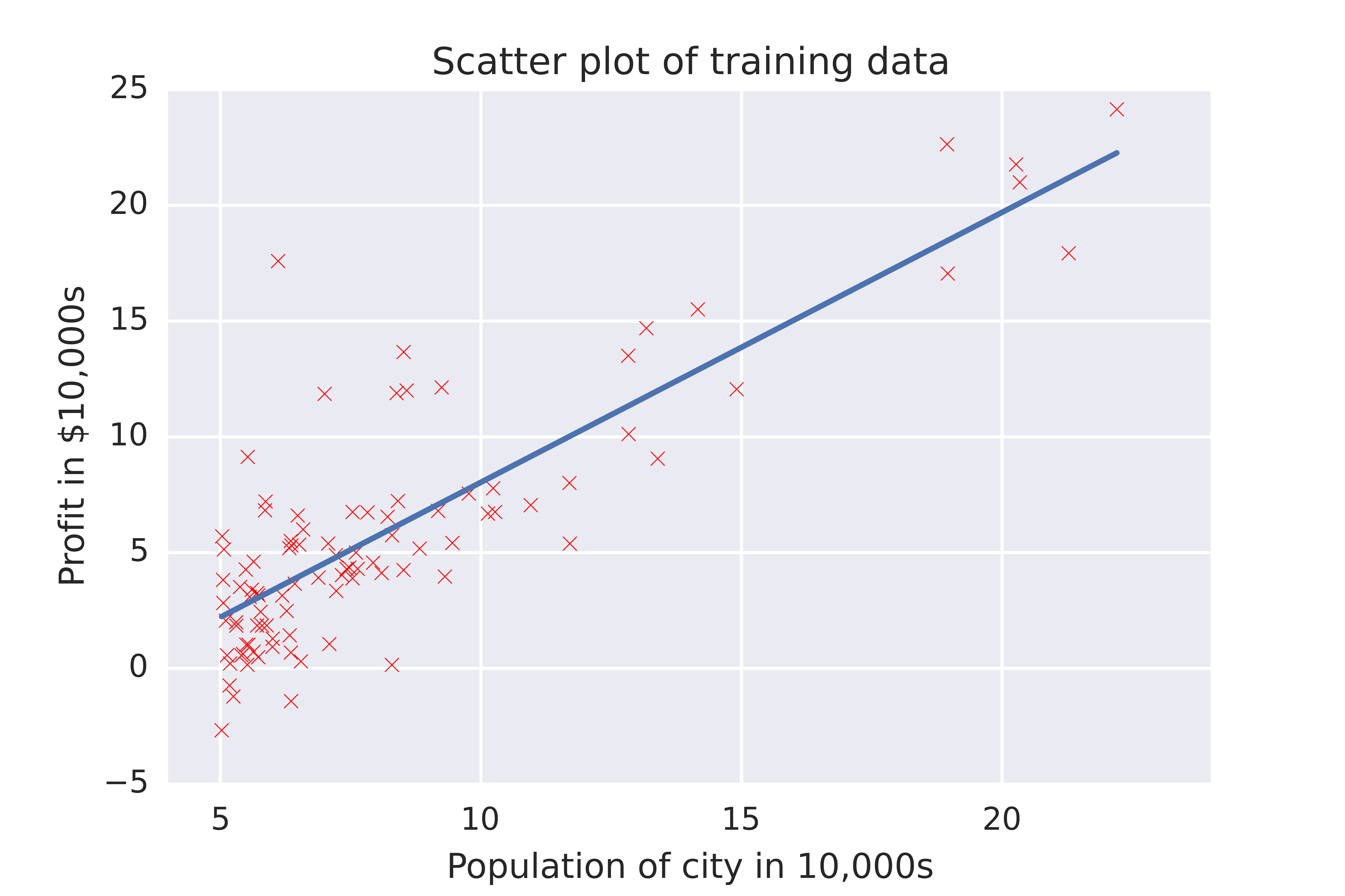
So, after all of that we end up with parameters of \(\theta_0\) and \(\theta_1\) that we can use to plot on our scatter graph.

Woo! Gradient descent was able to find values of \(\theta_0\) and \(\theta_1\) to fit a nice regression line to our data. Now we can predict that if we send food trucks to Cambridge, UK (population ~128,500 during term time), we’ll make ~$113574, whereas if we open up shop in Cambridge, MA (population ~107,300), we can expect to make ~$88,847.
I hope that this was a useful introduction to gradient descent. You can see my code here. We can also use gradient descent for multivariate linear regression (I won’t go into this here, maybe in another post). I expect we’ll be using variations of this algorithm for other applications later in the course, since it seems to be a machine learning staple.